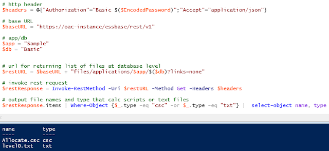
Moving on to the second part where I am looking at a possible solution to capturing and handling rejections in EPM Cloud Data Management.
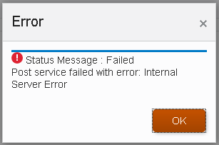
Just a quick recap on the first part, data was loaded through Data Management but there were records rejected due to missing entity members in the target application. With help from scripting and the REST API I covered a method to run the data load rule, check the status of the load rule and if there was a failure then download the process log, the process log was parsed for data load rejections if any were found these were sent in an email.
![]()
In this post I am going to extend the process for capturing rejections and handle them by using the metadata functionality that is now available in Data Management.
Like in the previous part I will be focusing on the entity member rejections but there is nothing stopping expanding the process to handle other dimensions, though saying that if there are rejections across multiple dimensions then it might be best to concentrate on starting with a cleaner data source file.
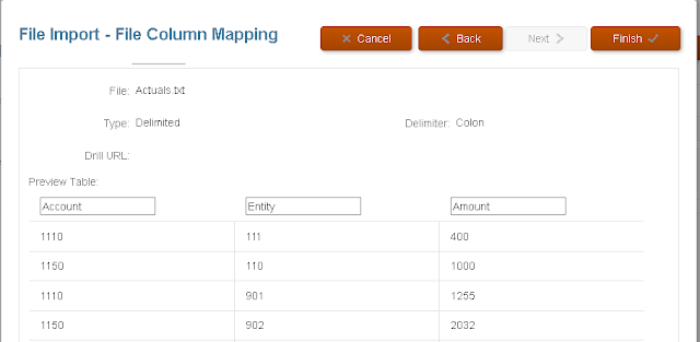
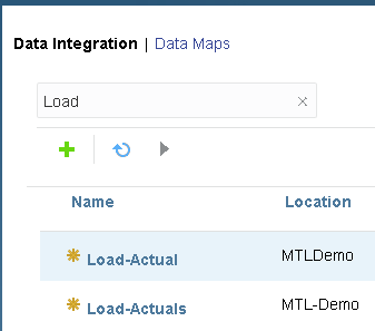
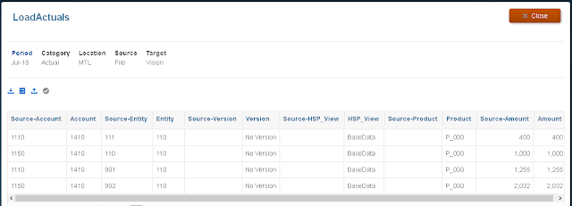
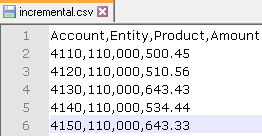
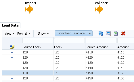
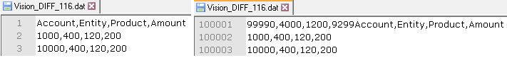
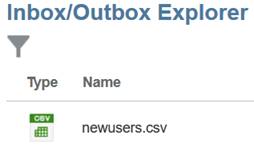
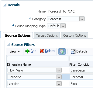
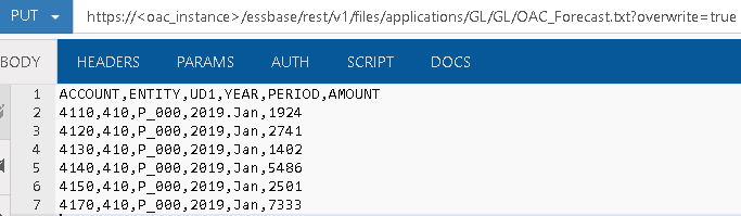
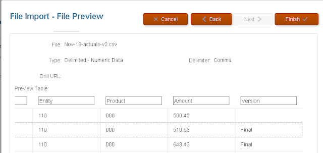
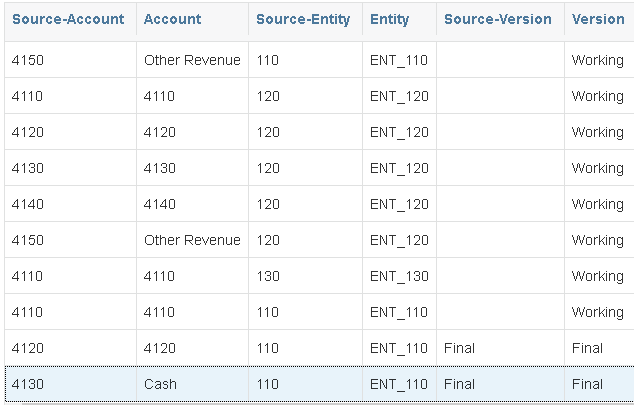
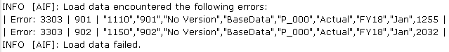
I am going to use the same source file where the rows containing entity members “901” and “902” will be rejected due the members not existing in the target application.
![]()
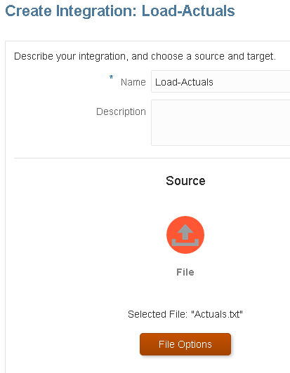
The aim will be to extract the rejected entity members from the process log and write them to a text file which can be uploaded to Data Management.
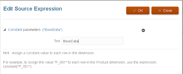
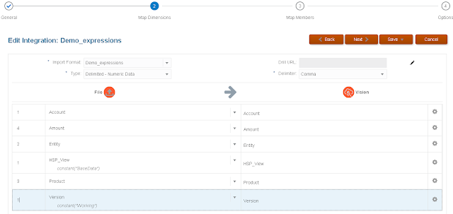
Using a metadata load rule, the members will be loaded based on mapping logic, so in this example they will be loaded as children of “900”.
![]()
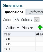
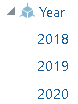
Even though I am not yet a fan of the simplified dimension editor I thought I had better start using it in my examples as the classic editor is no longer going to be supported.
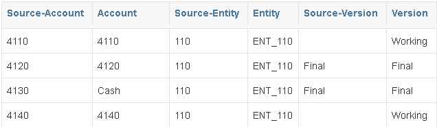
Once the members have been loaded and a refresh performed, the data load can be run again and there should be no rejections.
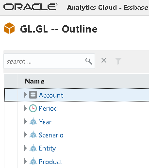
Before we can get to that stage a metadata load needs to be setup in Data Management, I am not going to go into great detail around the metadata functionality as I have already covered this topic in a previous blog which you can read all about here.
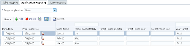
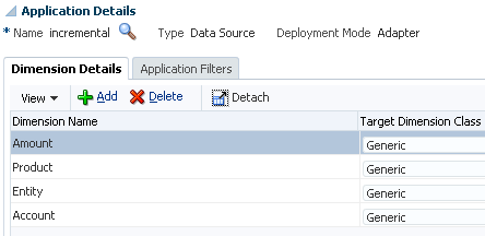
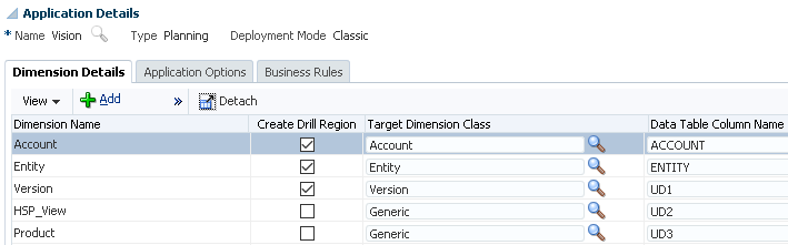
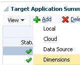
Under the Target Application Summary dimensions are added.
![]()
For the entity dimension I have only enabled the properties I will be using in the metadata load, these are parent, member and data storage. I could have got away with not including data storage and let the system pick the default value but I just wanted to show that properties that are not contained in the source can be included.
![]()
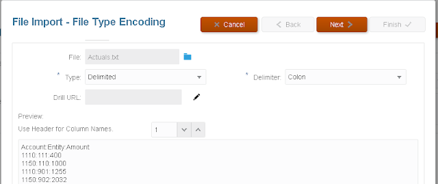
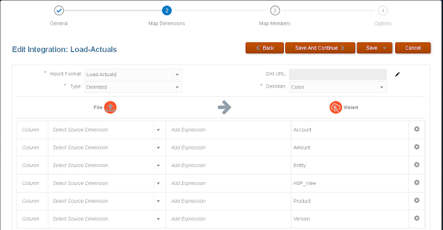
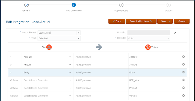
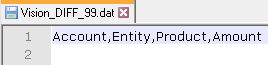
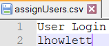
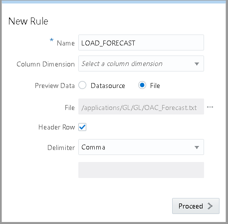
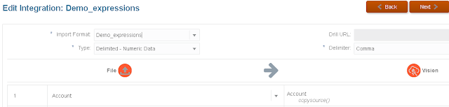
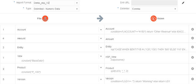
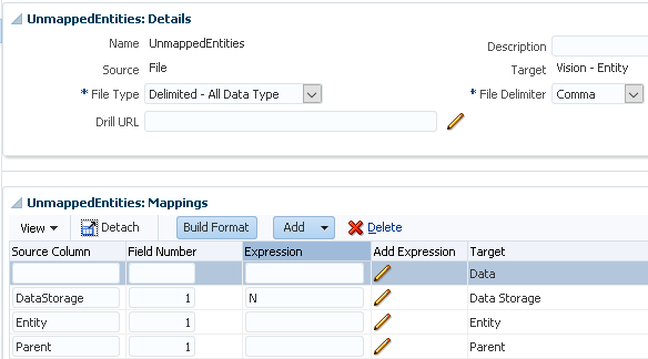
The import format is simple as the source file will only have one column containing the new entity members.
The File Type should be set as “Delimited – All Data Type” and the Data column is ignored for metadata loads.
![]()
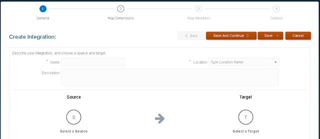
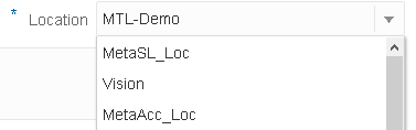
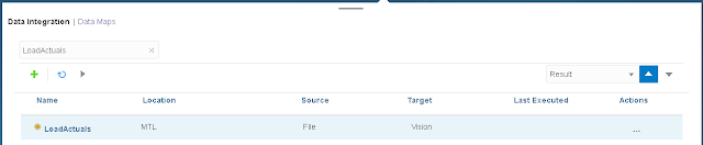
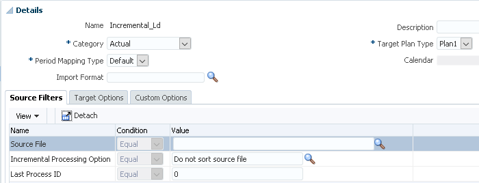
A new location was added and a new data load rule created against the new location.
I assigned to a category named “Metadata” which I have for metadata type loads.
![]()
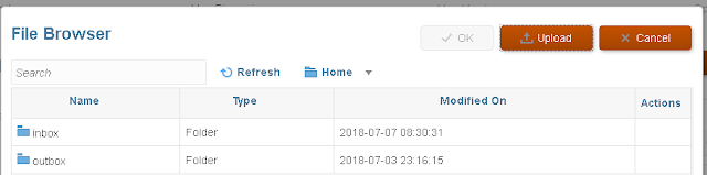
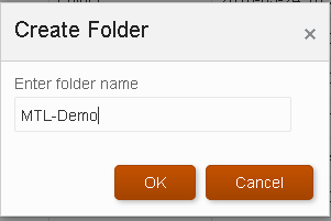
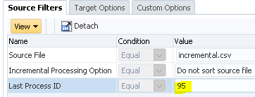
I did not set a file as I am going to include that in the automation script, the directory was defined as the location folder where the script will upload the rejected member file to.
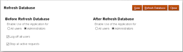
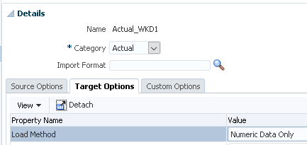
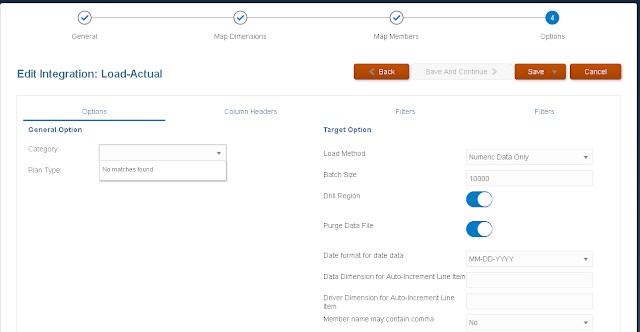
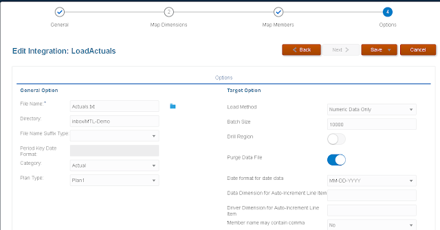
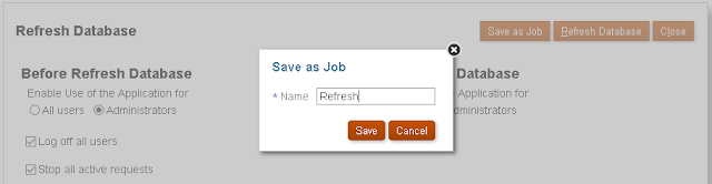
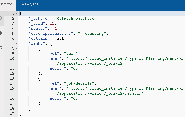
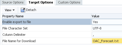
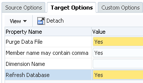
In the target options of the rule the “Refresh Database” property value was set to “Yes” as I want the members to exist in Essbase when the data is reloaded.
![]()
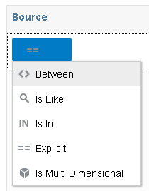
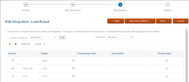
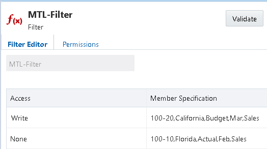
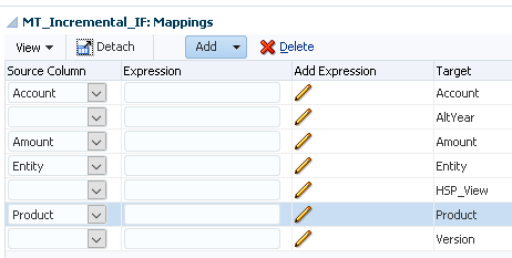
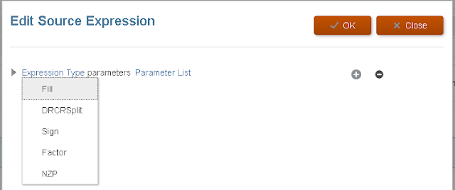
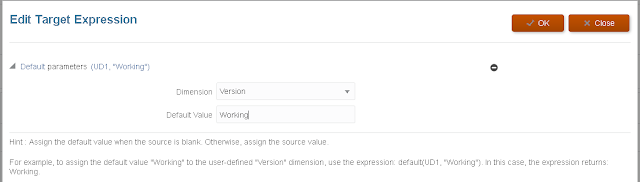
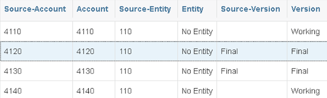
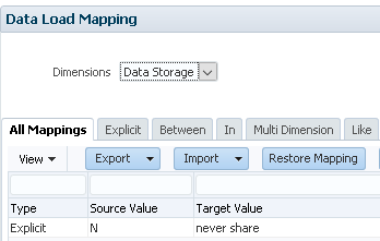
On to the mappings, an explicit mapping is defined for “Data Storage” to map “N” from the import format to “never share”.
![]()
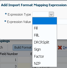
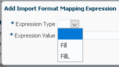
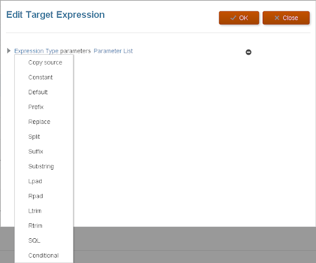
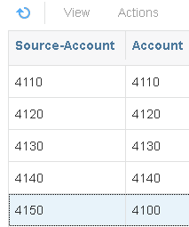
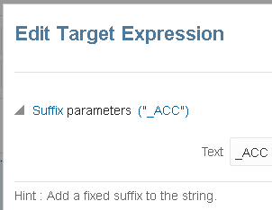
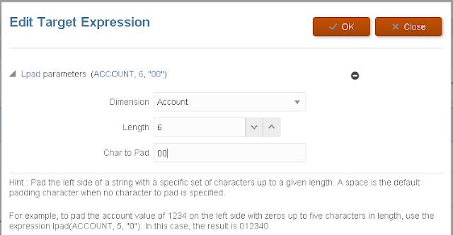
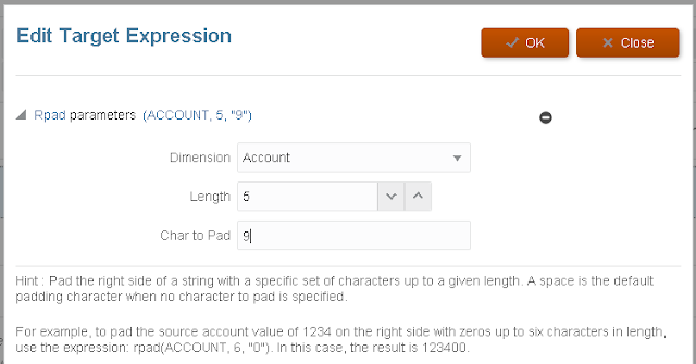
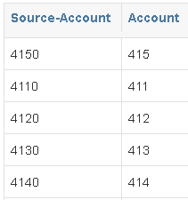
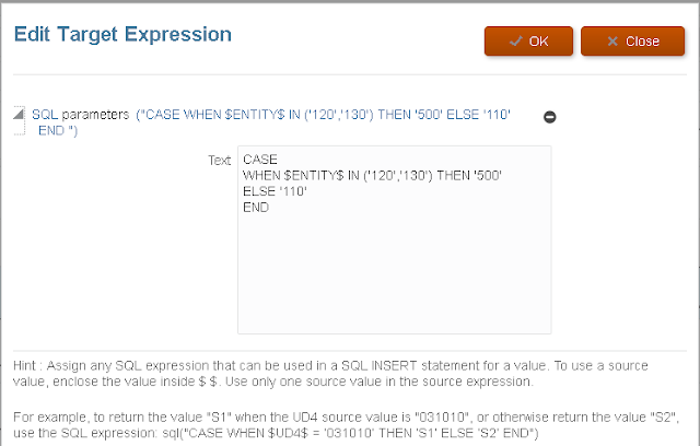
For the parent I used a “#FORMAT” mapping type which will take the first character of the member and then suffix “00”, if you look back I also mapped the entity member to parent, so as an example member “901” will be mapped to the parent “900”
![]()
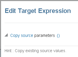
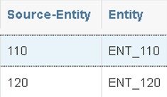
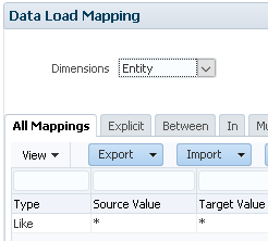
The entity member property was defined as a like for like mapping, this is because I want the source member to be the same as the target.
![]()
If I wanted to expand the automation process further I could add in a step to upload explicit mappings for the new entity members.
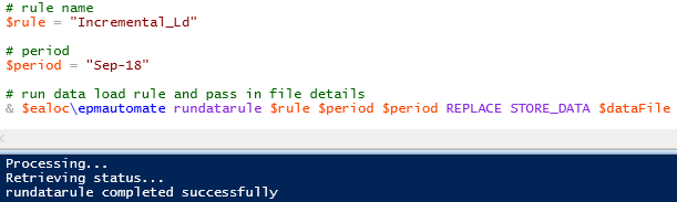
Now the rule is in place it is time to go back to my original PowerShell script from the last blog post and modify it to handle the metadata load.
I am going to continue with the script from the point where the process log has been downloaded, this means the data load has taken place and failed.
In the last part I parsed the process log and added any rejections to an email, this time I am going to parse and create a file with the rejected members in.
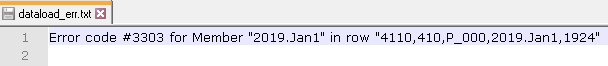
In the process log the rejected rows of data will contain “Error: 3303”.
![]()
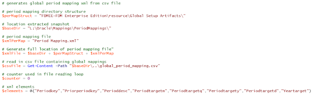
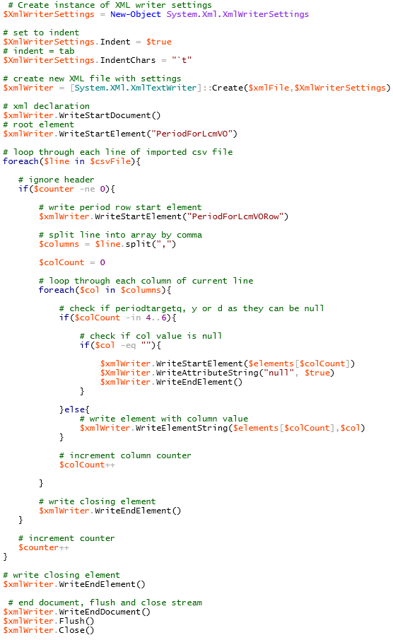
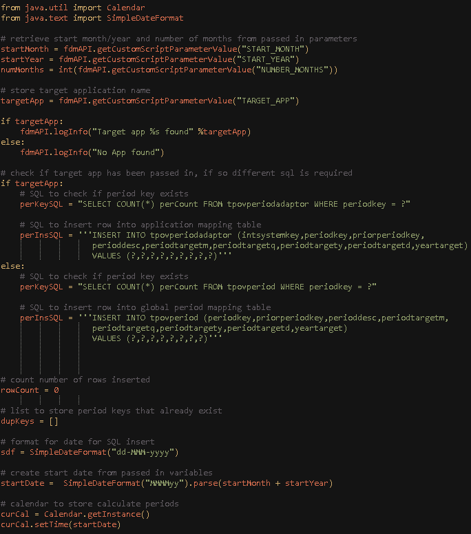
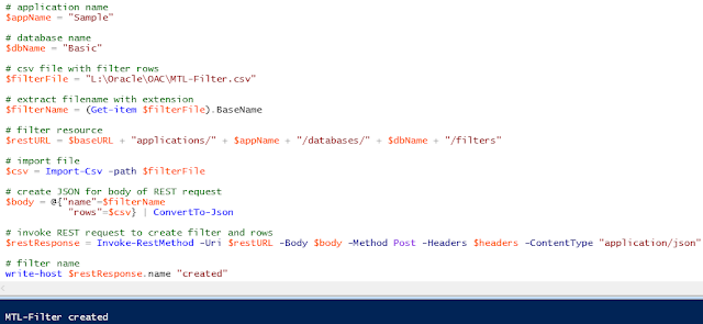
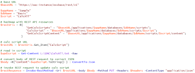
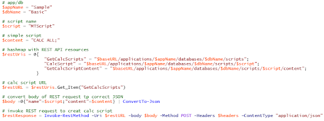
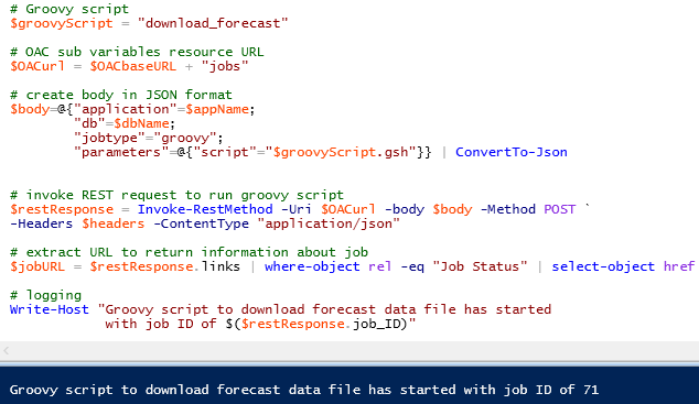
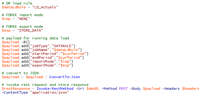
I will break the script into bite sized sections and include the variables which usually would be at the start of the script.
![]()
The variables above have comments so I shouldn’t need to explain them but I have cut down on the number of variables for demo purposes in this post, the final script includes variables where possible and functions to stop repetition.
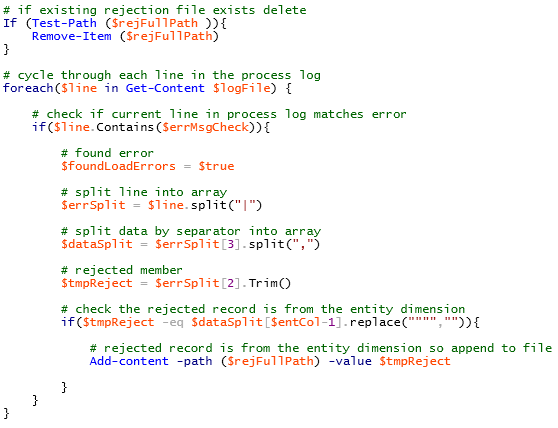
On to the next section of the script which checks if there is an existing entity rejection file, if there is, delete.
Each line of the process log is then cycled through and if a line contains “Error: 3303” then it is parsed to extract the entity member, the script could be enhanced to handle multiple dimensions but I am trying to keep it simple for this example.
![]()
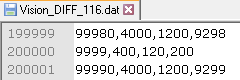
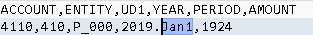
To break down the parsing section further let me take the following line as an example:
![]()
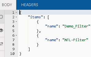
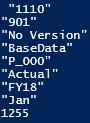
First the line is split by a pipe delimiter and stored in an array, for the above the array would look like:
![]()
The second entry in the array contains the member that was rejected, the third entry contains the data record.
The data record is then split by a comma delimiter and stored in an array which looks like.
![]()
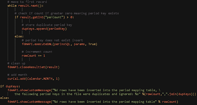
A test is then made to confirm that the rejected member is part of the entity dimension as that has been defined as the second entry in the data record, if they match the member is then appended to the entity rejection file.
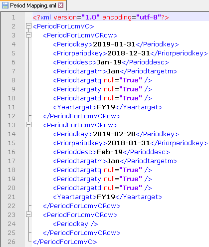
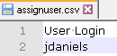
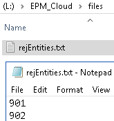
Now I have a file containing all the rejected entity members.
![]()
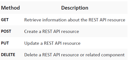
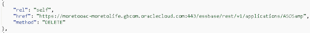
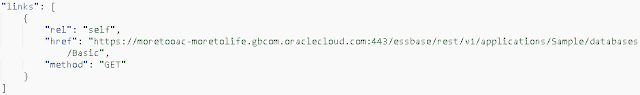
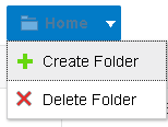
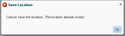
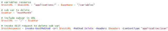
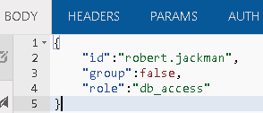
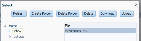
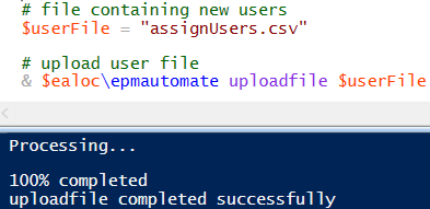
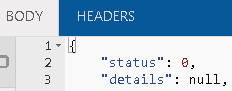
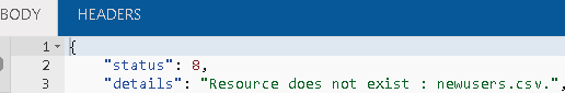
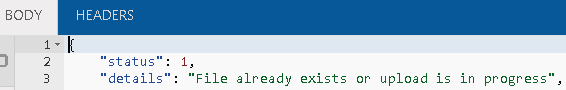
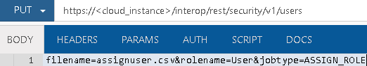
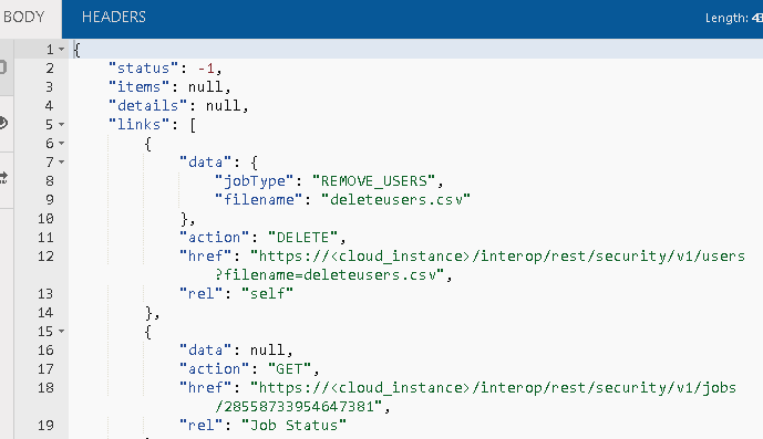
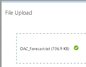
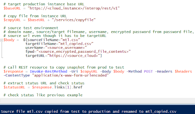
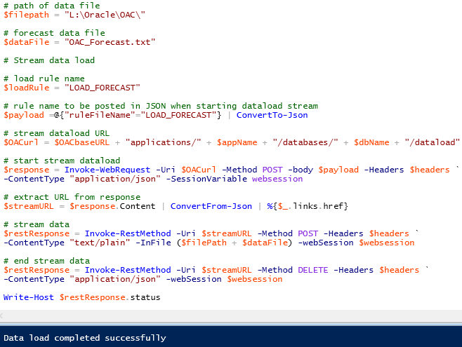
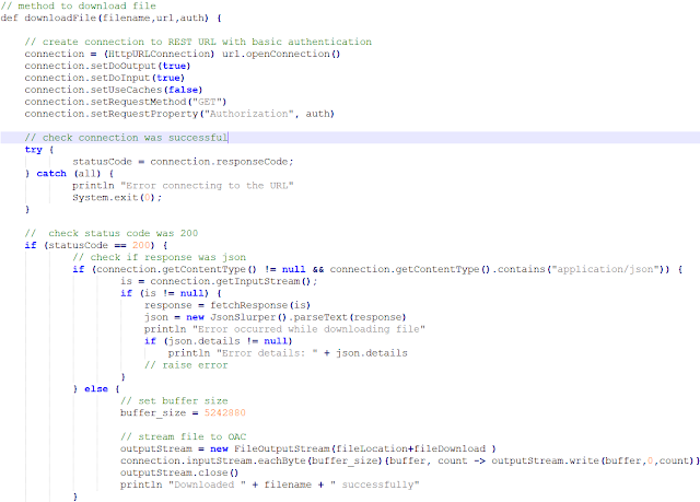
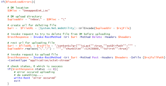
Using the REST API, the file can be uploaded to the location directory in Data Management, as there could be an existing file in the directory with the same name, the delete REST resource is used to remove the file, it doesn’t matter if the file does not exist.
![]()
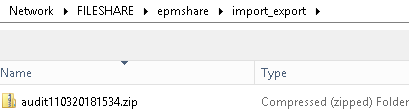
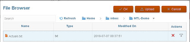
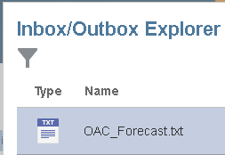
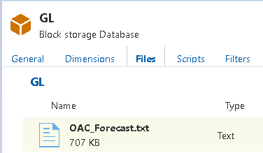
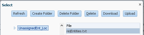
After this section of the script has run, the entity rejection file should exist in the Data Management location folder.
![]()
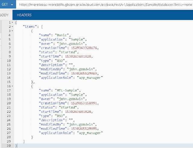
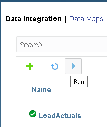
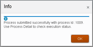
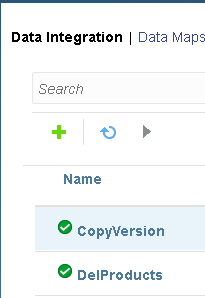
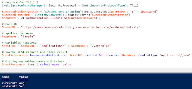
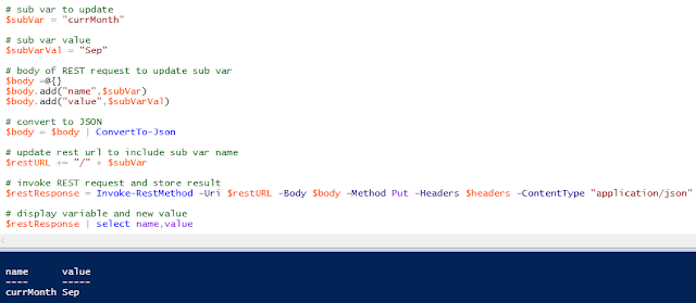
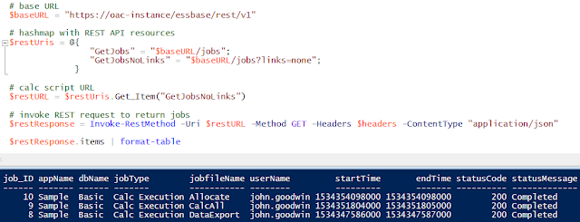
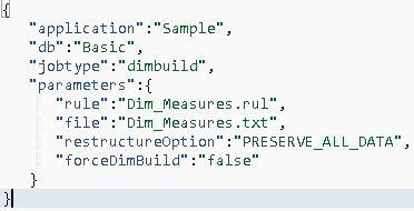
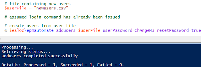
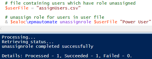
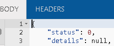
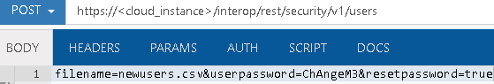
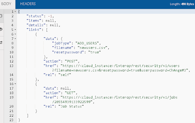
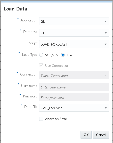
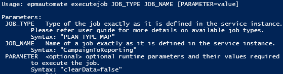
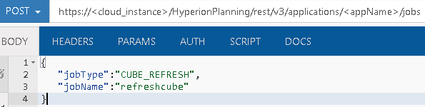
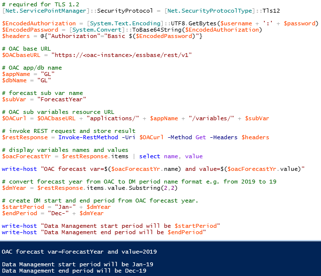
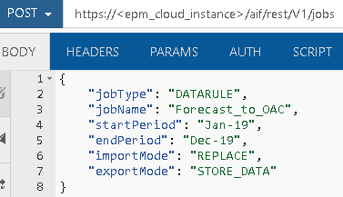
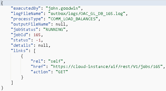
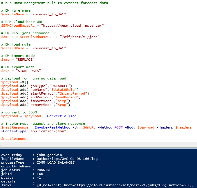
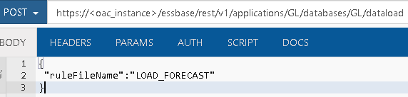
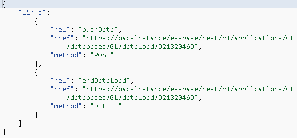
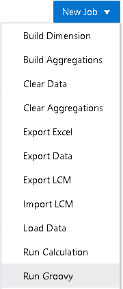
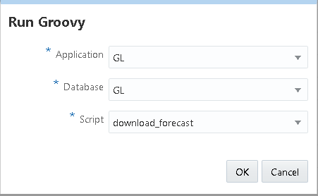
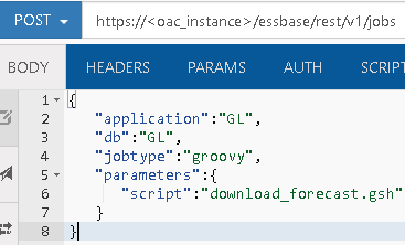
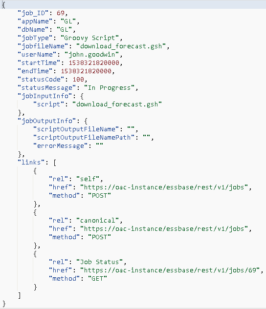
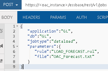
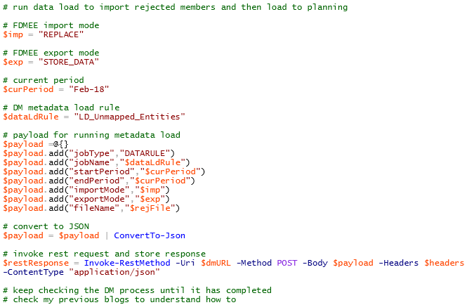
Next the REST API comes into play again to run the metadata load rule that I created earlier in Data Management.
![]()
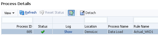
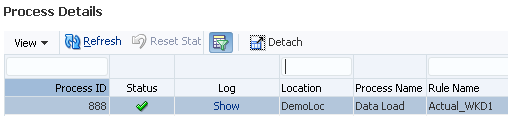
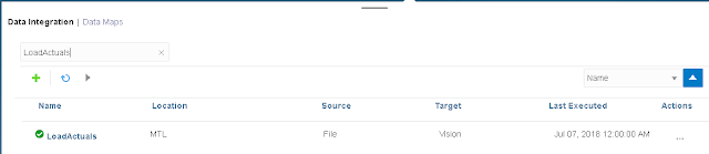
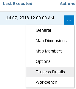
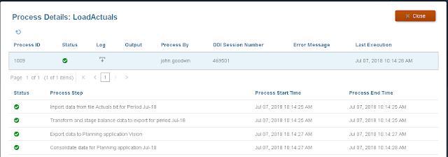
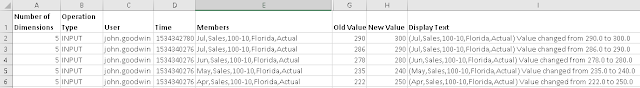
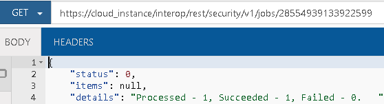
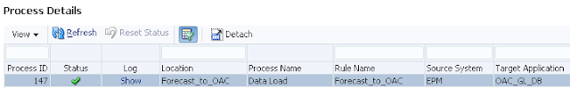
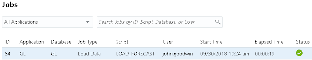
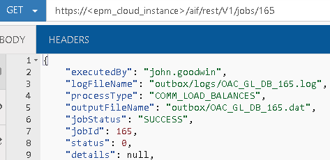
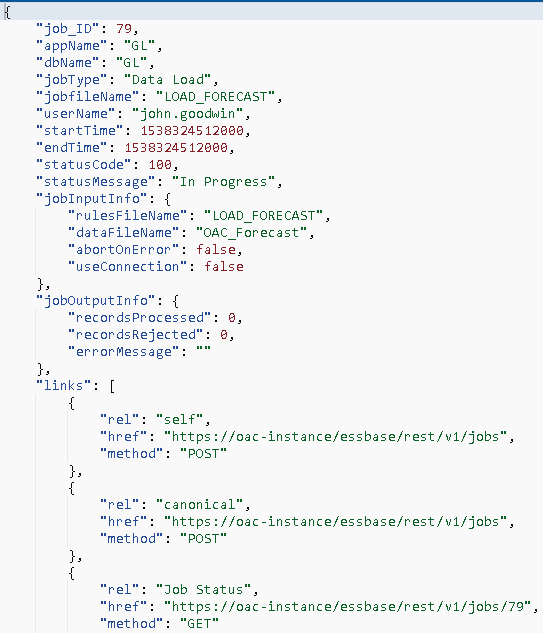
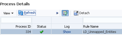
At this point, if I check process details in Data Management it shows that metadata rule has successfully completed.
![]()
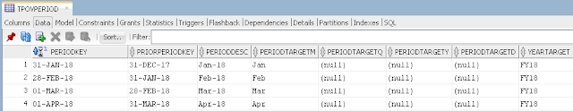
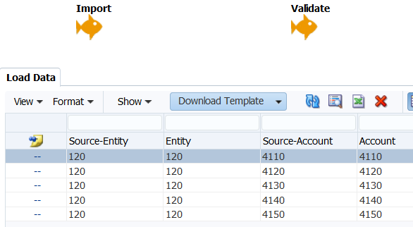
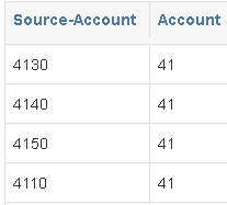
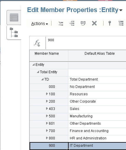
In the workbench you can see that entity members have been mapped to the correct parent.
![]()
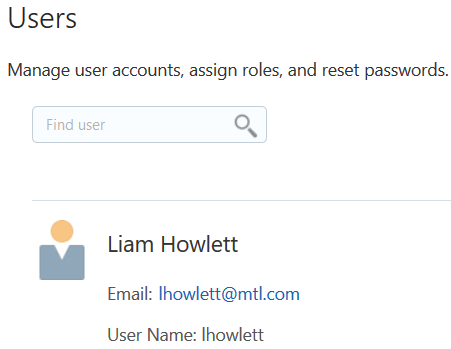
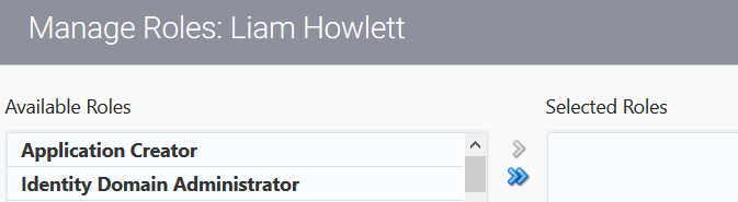
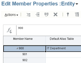
Within the target application the entity members have been successfully loaded.
![]()
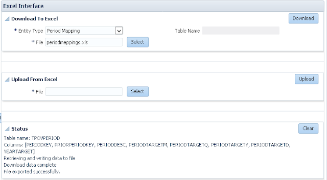
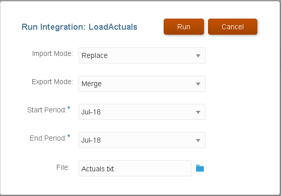
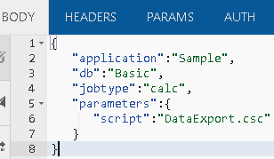
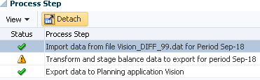
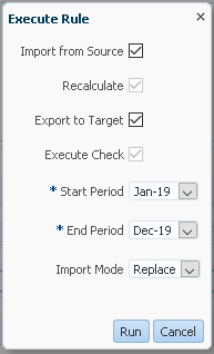
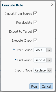
As the metadata has been loaded and pushed to Essbase the export stage of the data load rule can be run again.
![]()
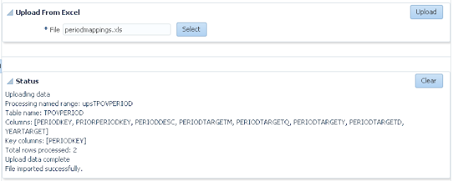
This time the data load was successful
![]()
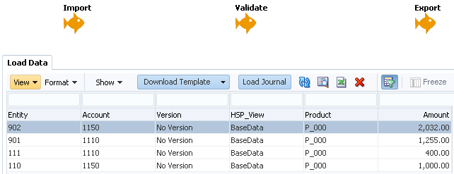
The workbench confirms all rows of data have been loaded to the target application.
![]()
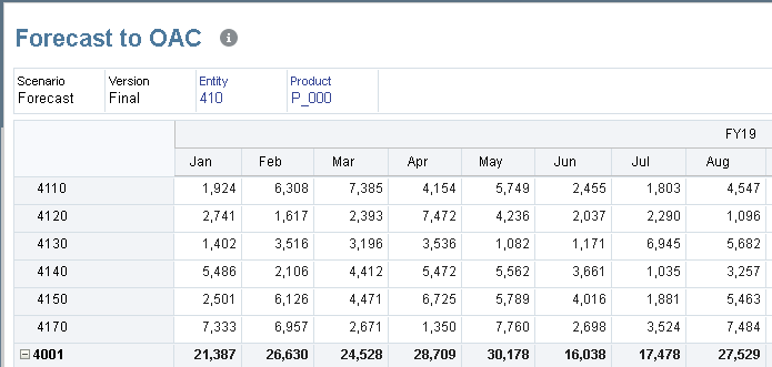
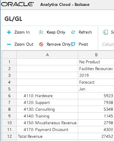
A quick retrieve verifies the data is definitely in the target application.
![]()
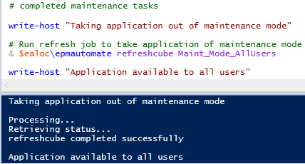
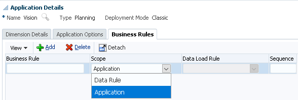
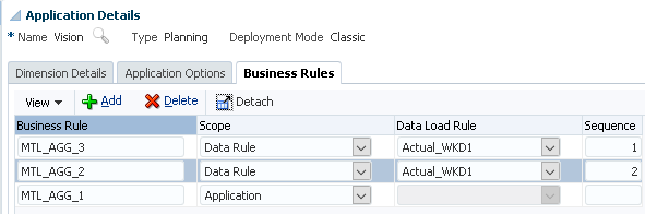
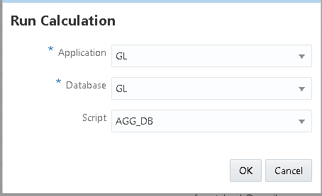
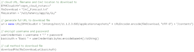
After the data load has successfully completed, a step could have been added to run a rule to aggregate the data, once again this can be achieved by calling a REST resource which I have covered in the past.
A completion email could then be sent based on the same concept shown in the previous blog post.
![]()
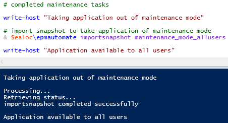
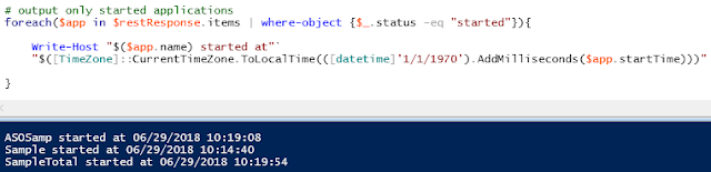
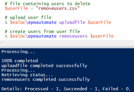
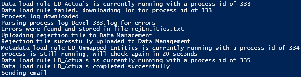
An example of the output from the full automated process would be:
![]()
So there we go, an automated data load solution that captures and handles rejections. If you are interested in a similar type of solution then please feel free to get in touch.
Just a quick recap on the first part, data was loaded through Data Management but there were records rejected due to missing entity members in the target application. With help from scripting and the REST API I covered a method to run the data load rule, check the status of the load rule and if there was a failure then download the process log, the process log was parsed for data load rejections if any were found these were sent in an email.

Like in the previous part I will be focusing on the entity member rejections but there is nothing stopping expanding the process to handle other dimensions, though saying that if there are rejections across multiple dimensions then it might be best to concentrate on starting with a cleaner data source file.
I am going to use the same source file where the rows containing entity members “901” and “902” will be rejected due the members not existing in the target application.

The aim will be to extract the rejected entity members from the process log and write them to a text file which can be uploaded to Data Management.
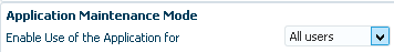
Using a metadata load rule, the members will be loaded based on mapping logic, so in this example they will be loaded as children of “900”.
Even though I am not yet a fan of the simplified dimension editor I thought I had better start using it in my examples as the classic editor is no longer going to be supported.
Once the members have been loaded and a refresh performed, the data load can be run again and there should be no rejections.
Before we can get to that stage a metadata load needs to be setup in Data Management, I am not going to go into great detail around the metadata functionality as I have already covered this topic in a previous blog which you can read all about here.
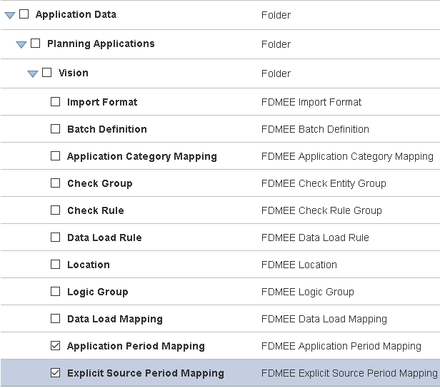
Under the Target Application Summary dimensions are added.
For the entity dimension I have only enabled the properties I will be using in the metadata load, these are parent, member and data storage. I could have got away with not including data storage and let the system pick the default value but I just wanted to show that properties that are not contained in the source can be included.

The import format is simple as the source file will only have one column containing the new entity members.
The File Type should be set as “Delimited – All Data Type” and the Data column is ignored for metadata loads.
A new location was added and a new data load rule created against the new location.
I assigned to a category named “Metadata” which I have for metadata type loads.
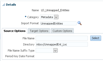
I did not set a file as I am going to include that in the automation script, the directory was defined as the location folder where the script will upload the rejected member file to.
In the target options of the rule the “Refresh Database” property value was set to “Yes” as I want the members to exist in Essbase when the data is reloaded.
On to the mappings, an explicit mapping is defined for “Data Storage” to map “N” from the import format to “never share”.
For the parent I used a “#FORMAT” mapping type which will take the first character of the member and then suffix “00”, if you look back I also mapped the entity member to parent, so as an example member “901” will be mapped to the parent “900”

The entity member property was defined as a like for like mapping, this is because I want the source member to be the same as the target.
If I wanted to expand the automation process further I could add in a step to upload explicit mappings for the new entity members.
Now the rule is in place it is time to go back to my original PowerShell script from the last blog post and modify it to handle the metadata load.
I am going to continue with the script from the point where the process log has been downloaded, this means the data load has taken place and failed.
In the last part I parsed the process log and added any rejections to an email, this time I am going to parse and create a file with the rejected members in.
In the process log the rejected rows of data will contain “Error: 3303”.
I will break the script into bite sized sections and include the variables which usually would be at the start of the script.

The variables above have comments so I shouldn’t need to explain them but I have cut down on the number of variables for demo purposes in this post, the final script includes variables where possible and functions to stop repetition.
On to the next section of the script which checks if there is an existing entity rejection file, if there is, delete.
Each line of the process log is then cycled through and if a line contains “Error: 3303” then it is parsed to extract the entity member, the script could be enhanced to handle multiple dimensions but I am trying to keep it simple for this example.
To break down the parsing section further let me take the following line as an example:

First the line is split by a pipe delimiter and stored in an array, for the above the array would look like:

The second entry in the array contains the member that was rejected, the third entry contains the data record.
The data record is then split by a comma delimiter and stored in an array which looks like.
A test is then made to confirm that the rejected member is part of the entity dimension as that has been defined as the second entry in the data record, if they match the member is then appended to the entity rejection file.
Now I have a file containing all the rejected entity members.
Using the REST API, the file can be uploaded to the location directory in Data Management, as there could be an existing file in the directory with the same name, the delete REST resource is used to remove the file, it doesn’t matter if the file does not exist.
After this section of the script has run, the entity rejection file should exist in the Data Management location folder.
Next the REST API comes into play again to run the metadata load rule that I created earlier in Data Management.
At this point, if I check process details in Data Management it shows that metadata rule has successfully completed.
In the workbench you can see that entity members have been mapped to the correct parent.

Within the target application the entity members have been successfully loaded.
As the metadata has been loaded and pushed to Essbase the export stage of the data load rule can be run again.
This time the data load was successful

The workbench confirms all rows of data have been loaded to the target application.
A quick retrieve verifies the data is definitely in the target application.

After the data load has successfully completed, a step could have been added to run a rule to aggregate the data, once again this can be achieved by calling a REST resource which I have covered in the past.
A completion email could then be sent based on the same concept shown in the previous blog post.

An example of the output from the full automated process would be:
So there we go, an automated data load solution that captures and handles rejections. If you are interested in a similar type of solution then please feel free to get in touch.